Linear models use within-month rank features, while tree-based models use raw winsorized inputs. Time-based splits (training pre-2012, validation 2012–2018, test 2019–2024) support clean out-of-sample (OOS) model comparison, and the final PRIM valuation refits the winning models on the full 645,595-observation modeling sample.
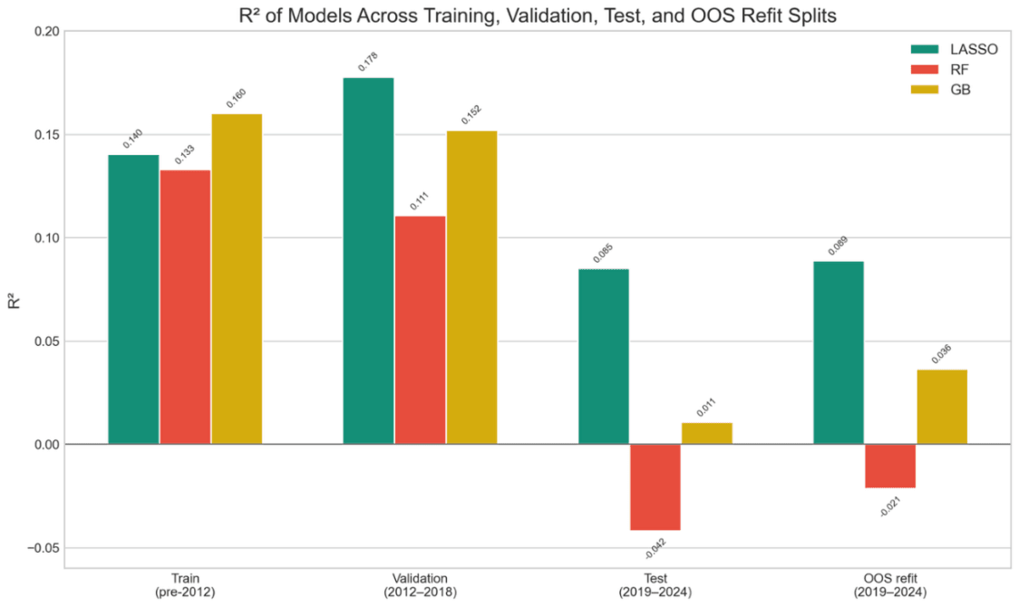
Among linear models, LASSO matches OLS out-of-sample at an R² of 8.9%, confirming the OLS model. Among tree-based methods, gradient boosting outperforms random forest (3.6% vs −2.1% OOS R²), consistent with a fairly smooth and stable relationship between fundamentals and valuation. A 50/30/20 blend of LASSO, gradient boosting, and random forest yields a fair-value P/E of 20.54x, compared with an actual forward two-year P/E of 16.08x implied by PRIM’s October 31, 2024 share price and forward earnings estimates. This represents roughly a 22% discount, suggesting moderate undervaluation on fundamentals. The three models produce very similar estimates, all within a 0.8-turn range, and using equal weights gives 20.65x, showing the result does not depend much on the exact weighting. Since the model is built only on observable fundamentals and leaves out other drivers like market sentiment or firm-specific developments, the gap is better viewed as a general indication of moderate undervaluation than a precise measure of mispricing.
Introduction
This report estimates a fair-value forward two-year price-to-earnings (P/E) multiple for Primoris Services Corporation (PRIM) as of October 31, 2024. PRIM is a specialty infrastructure contractor in the GICS Capital Goods Industry Group (2010), operating through the Utilities and Energy segments. Utilities focuses on power delivery and gas across the United States, while Energy operates in the United States and Canada and provides engineering, procurement, construction, and maintenance services for renewables, energy infrastructure, and related end markets. In recent years, its revenue mix has shifted away from pipeline-heavy construction toward utility-scale renewables and electric power delivery.
I estimate PRIM’s industry-adjusted earnings yield using a large sample of 648,246 firm-month observations from January 2001 to October 2024. The earnings yield for each firm is the ratio of the consensus analyst EPS estimate two years ahead to the current share price. I apply five models that range from simple linear specifications to more complex tree-based methods: ordinary least squares, penalized regression (LASSO), a single decision tree, a random forest, and gradient boosting. Predictions from the three best-performing models are combined and added back to the industry-group earnings yield to produce a fair-value multiple, which is then compared to PRIM’s actual trading multiple as of October 31, 2024.
Data
Variables
The dependent variable is the industry-adjusted earnings yield, computed as the firm’s forward two-year earnings yield less the industry group mean. Table 1 lists the continuous variables with brief descriptions; the appendix expands on each. Book-to-market equity is excluded because it is itself a valuation ratio and overlaps with the dependent variable. It is replaced with analyst sales growth forecasts, which capture the growth expectations embedded in earnings yield, where higher growth is associated with lower yields and higher P/E multiples.
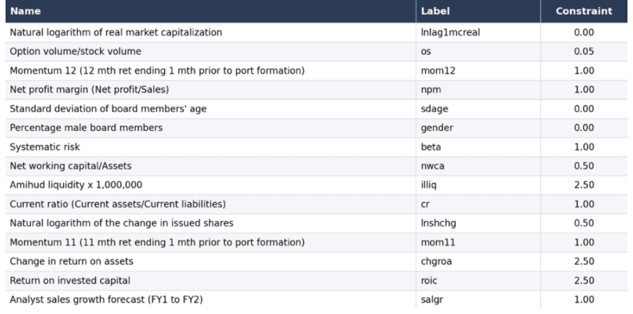
I begin with 15 continuous candidate predictors, which I narrowed down through a pairwise correlation screen for redundancy using the Pearson correlation coefficient (ρ). At ρ > 0.60, variables largely duplicate the same signal, so I retain the one with broader economic coverage:
- mom12 kept over mom11 (ρ = 0.94): Twelve-month returns are the standard momentum horizon in practice, so mom12 is the more conventional choice.
- gender kept over sdage (ρ = 0.71): Gender share varies more across firms’ board members, giving it more power to differentiate them.
- cr kept over nwca (ρ = 0.62): Current ratio focuses on short-term assets and liabilities, while net working capital to assets mixes liquidity with a firm-size effect from total assets.
After these drops the maximum remaining pairwise ρ is 0.38, within a stable-estimation range. The final feature set is 12 continuous predictors plus 10 missingness indicators, for 22 total features.
Descriptive Statistics
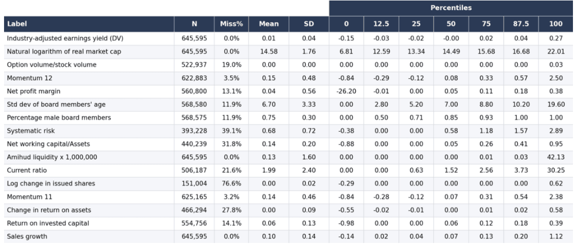
The modeling sample contains 645,595 firm-month observations after excluding the final cross-section used for the PRIM prediction. Table 2 reports the mean, standard deviation, and percentile distribution of the dependent variable and the fifteen continuous candidate predictors on this sample, with per-variable N and Miss% calculated relative to the total.
Primoris Services’ Position in the Sample
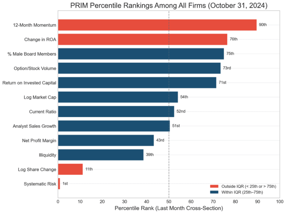
In the October 31, 2024 cross-section PRIM ranks in the 90th percentile for 12-month momentum, the 76th percentile for the month-on-month change in return on assets, the 71st percentile for return on invested capital, and the 1st percentile for beta (Figure 1). Together, high momentum, low systematic risk, and strong and improving profitability describe PRIM’s profile going into the estimation; the model will translate this profile into a fair-value earnings yield and P/E multiple.
Sample Split
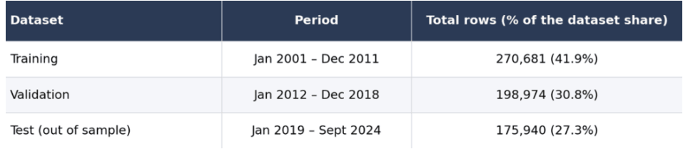
All models use a shared sample design. I reserve firm-months before January 2012 as the training set, months from January 2012 through December 2018 as the validation set, and months from January 2019 through September 2024 as the test set. For the headline out-of-sample (OOS) result, I refit the model on all data prior to the test period (pre-2019) and evaluate it on the test period (January 2019 to September 2024). For the final PRIM prediction, I refit on the full modeling sample, so the estimate reflects all available history through September 2024, with October 31, 2024 reserved as the target cross-section. All splits are time-based rather than random to avoid lookahead and match the information set available in real time.
Results
Regression
I begin with linear cross-sectional regressions to relate firm characteristics to industry-adjusted earnings yield. Linear models use within-month cross-sectional ranks scaled to [0,1]. This removes level drift over time and captures monotonic effects, allowing the model to pick up most of the economic relationships.
Ordinary Least Squares (OLS) Regression
The OLS regression on all 22 rank features yields strong, economically meaningful relationships, with coefficients aligning with standard valuation predictors. Most notably, moving from the lowest to the highest lagged market capitalization lowers industry-adjusted earnings yield by 8.8 percentage points (t = −144); return on invested capital raises it by 3.5 percentage points (t = 134); and 12-month momentum lowers it by 1.9 percentage points (t = −104). Together, this points to larger firms with strong capital productivity and positive price momentum. The OLS PRIM prediction is an industry-adjusted earnings yield of 0.15%, which, added to the Capital Goods industry-group mean earnings yield of 4.75%, gives a total earnings yield of 4.90%. Inverting that yield produces a P/E multiple of 20.38x.
Penalized Regression
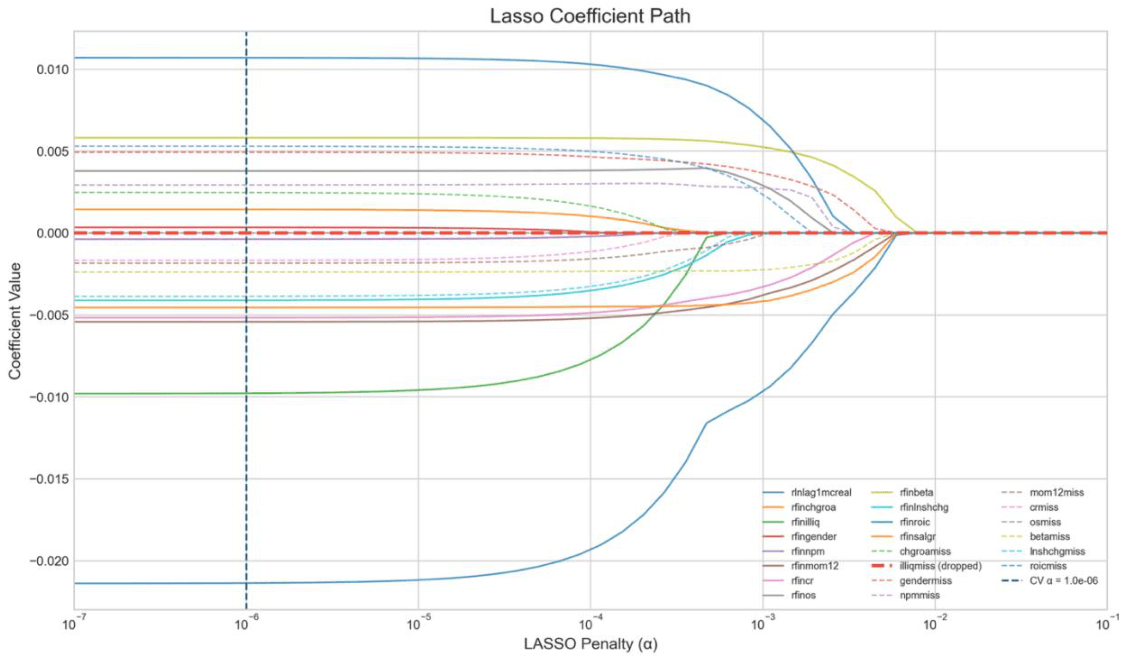
The Least Absolute Shrinkage and Selection Operator (LASSO) applies an L1 penalty that shrinks small coefficients to zero and performs variable selection. I fit the model with 5-fold cross-validation across penalty values (α) from 10⁻⁶ to 10⁻¹ on standardized rank features, and the cross-validated prediction error is minimized at α ≈ 10⁻⁶ (Figure 2), the lightest penalty on the grid. With 22 features and a large sample, the OLS estimates are already stable, leaving little scope for additional shrinkage to improve OOS performance. In this setting, LASSO serves less to reduce overfitting and more to confirm which signals remain robust under even minimal penalization. As the penalty gets stronger, the illiquidity missingness indicator is the first to fall to zero, followed by gender and net profit margin, while lagged market capitalization, return on invested capital, and Amihud illiquidity are the last to survive. At the selected penalty, only the illiquidity missingness indicator is dropped.
Among the retained variables, the largest standardized coefficients are lagged market capitalization (−0.021), return on invested capital (0.011), and Amihud illiquidity (−0.010). Translated back onto the rank scale, moving from the smallest to the largest lagged market capitalization lowers industry-adjusted earnings yield by 8.8 percentage points; moving from the lowest to the highest return on invested capital raises it by 3.5 percentage points; and moving from the least to the most illiquid stocks lowers it by 4.1 percentage points. Together, this points to lower earnings yields at larger firms with strong cash generation and deeper trading liquidity, consistent with the OLS results.
In Table 4, both models have identical R² across all three evaluation windows: 17.8% on the 2012–2018 validation window, 8.5% on the 2019–2024 test window, and 8.9% on the OOS refit that adds the 2012–2018 data to the training set.
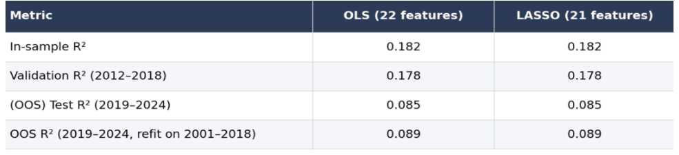
As a robustness check, refitting OLS and LASSO on the raw winsorized features instead of within-month ranks reduces OOS R² to 3.3%, indicating that the rank transformation nearly triples OOS fit. The LASSO PRIM prediction is an industry-adjusted earnings yield of 0.15%, giving a total yield of 4.90% and a P/E of 20.38x, within 0.01x of the OLS estimate.
Decision Trees
Tree-based models relax the linear assumptions of OLS and LASSO. Because these methods are largely unaffected by transformations like ranking, I revert to the original winsorized features, which preserve magnitude information without requiring additional scaling. I then move from a single regression tree to a random forest and finally to gradient boosting.
Vanilla Decision Tree
A single tree with a max depth of 4 and a minimum leaf size of 10% of the training set reaches a train R² of 8.4% and a validation R² of 6.8%, but delivers a test R² of −5.7%. It captures patterns in-sample that do not carry over OOS, reflecting the instability of a single tree and motivating ensemble methods that reduce variance and improve generalization. The PRIM prediction under the single decision tree is an industry-adjusted earnings yield of 0.45%, giving a total yield of 5.20% and a P/E of 19.21x.
Random Forest
Random forest builds many trees on different samples of the data and subsets of features, then averages their predictions to reduce noise and improve stability. I test 48 combinations of key parameters, including tree depth, minimum leaf size, the number of features considered at each split, and the share of data used for each tree, while keeping the number of trees fixed at 100, and select the setup that performs best on the 2012–2018 validation window. As shown in Figure 3, validation R² rises with deeper trees and smaller minimum leaves, with the best cells clustered around 11%; the winner uses a maximum depth of 9, a minimum leaf size of 5%, 10 candidate features per split, and a 30% row subsample.
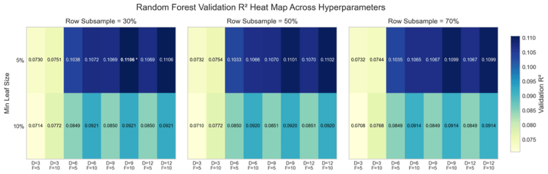
It delivers an in-sample R² of 13.3%, a validation R² of 11.1%, a test R² of −4.2% on the 2019–2024 window, and an OOS R² of −2.1%. Notably, none of the 48 configurations achieved a positive test R², suggesting that the shift between the train and test periods disrupts the tree’s decision rules more than it does the rank-based linear models.
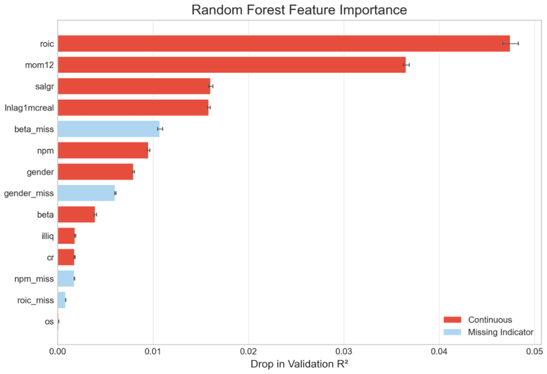
Figure 4 ranks the tuned random forest’s features by permutation importance, measured as the drop in validation R² when each feature’s column is randomly shuffled on the 2012–2018 window. This works by testing how much OOS accuracy falls when each input is disrupted. Return on invested capital and 12-month momentum dominate, responsible for a 4.7 and 3.7 percentage-point drop in validation R² respectively, with analyst sales growth and lagged market capitalization also contributing meaningfully at roughly 1.6 percentage points each. Return on invested capital and lagged market capitalization also appear among the largest standardized coefficients in the LASSO fit, so the same profitability and size factors carry the signal under two structurally different methods. The trees place more weight on momentum and less on illiquidity than LASSO, but the overlap in the core factor set is reassuring. The PRIM prediction under the random forest is an industry-adjusted earnings yield of −0.03%, giving a total yield of 4.72% and a P/E of 21.19x.
Gradient Boosting
Gradient boosting builds trees sequentially, where each new tree is trained on the residuals of the current model and is added in small steps using a learning rate that limits how much each tree can change the prediction. It uses the same type of trees as random forest, but instead of averaging many independent trees, it builds the model incrementally by correcting mistakes. I tune to relatively shallow trees and a smaller ensemble, with a maximum depth of 5, a minimum leaf size of 10%, 50 boosting rounds, six candidate features per split, a 60% row subsample, and a learning rate of 0.1, reflecting that each tree only needs to make a small incremental improvement. Gradient boosting dominates the random forest on every metric. It reaches an in-sample R² of 16.0%, a validation R² of 15.2%, a test R² of 1.1% on the 2019–2024 window, and an OOS R² of 3.6%. The PRIM prediction under gradient boosting is an industry-adjusted earnings yield of 0.15%, giving a total yield of 4.90% and a P/E of 20.40x.
Reconciliation of Results
LASSO ranks first with an OOS R² of 8.9%, followed by gradient boosting at 3.6% and random forest at −2.1% (Figure 5). Because LASSO captures the linear signal, OLS adds no incremental value, and the single decision tree is outperformed by both ensemble methods, so each is excluded from the comparison.
I blend LASSO, random forest, and gradient boosting rather than pick a single winner. Because these models learn in different ways, combining them reduces reliance on any one approach and improves stability. The weights are chosen based on performance: LASSO receives 50% as the strongest OOS model, gradient boosting 30% as the best tree-based method, and random forest 20%, below an equal weight of 33%, to reflect its weaker OOS fit while still adding diversification. The blended prediction implies an industry-adjusted earnings yield of 0.11%, which, added to the Capital Goods industry-group yield of 4.75%, gives a total earnings yield of 4.86% and a fair-value P/E of 20.54x (Figure 6). An equal-weight blend yields 20.65x, so the result is largely unchanged across reasonable weight choices.
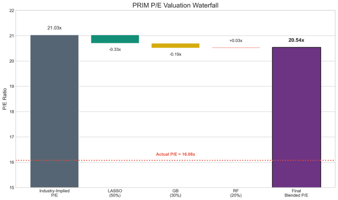
The actual P/E of 16.08x, implied by PRIM’s October 31, 2024 share price and mean analyst EPS forecasts two fiscal years ahead, sits roughly 22% below the blended fair-value P/E of 20.54x. This suggests PRIM is priced moderately below what the model’s cross-sectional fundamentals would predict.
Conclusion
The headline finding is that PRIM trades at an approximately 22% discount to its model-implied fair value, indicating moderate undervaluation. Using ranked inputs instead of raw values nearly triples OOS accuracy for the linear model, with R² rising from 3.3% to 8.9%. Tree-based models on the raw data capture less of the signal, with R² of 3.6% for gradient boosting and −2.1% for random forest. Taken together, this suggests the relationships are fairly consistent across firms and mostly move in one direction, which the rank-based linear model captures more effectively than the alternatives. Gradient boosting, which builds the model step by step, is able to recover part of this structure, but with lower accuracy. Random forest performs poorly out of sample, with no specification achieving a positive test R², indicating that its decision rules do not hold up well across time under this sample split. The model only captures a defined set of financial characteristics and not influences like sentiment or firm-specific risks, so the discount is best read as a directional signal of moderate undervaluation rather than a precise mispricing estimate.
Appendix
Real market capitalization and its natural logarithm
Real market capitalization is the market value of the stock, adjusted to purchasing power of November 2025 using the Consumer Price Index. There is a substantial body of evidence that small stocks have historically earned higher returns than large stocks (for example, Fama and French, 1992). This is most likely because small stocks are riskier than large stocks. Compared to companies with large market capitalization, small capitalization companies are likely to have less analyst coverage, less chance their debt is rated by ratings agencies like S&P, Moody’s and Fitch, less institutional investment and lower liquidity. Market capitalization is compiled from the CRSP database accessed via WRDS. The natural logarithm of real market capitalization is simply a transformation of real market capitalization for regression analysis to allow for a more realistic linear relationship between industry-adjusted stock returns and the market value of equity. Stocks listed in North America, and indeed most equity markets, have a small percentage of very large companies and a high percentage of medium and small companies.
Option volume/stock volume
The option to stock (O/S) volume ratio is the total monthly trading volume of all listed options on a firm’s stock divided by the total monthly trading volume of the firm’s stock. Option volume is the sum of all call and put options, regardless of strike price or maturity date. There is strong evidence that firms with high O/S ratios will earn lower returns relative to firms with a low O/S ratio (Johnson and So, 2012). This relationship is driven by the information advantage experienced in the options market. Options provide higher leverage, a limited downside risk, and lower cost option for traders wishing to act on negative private information. This is relevant when compared to short selling equities which require high borrowing fees and regulatory oversight. With this, informed traders tend to migrate to the options market ahead of adverse price movements. The O/S ratio reflects negative private information before it is incorporated into stock prices. However, increased institutional awareness of options-based indicators may have eroded some of its predictive power over time. The O/S ratio was constructed using data from the OptionsMetrics and CRSP databases on WRDS, covering all available firms between January 1996 and August 2025.
Momentum12 (12-month return ending 1 month prior to portfolio formation)
We use 12–1 momentum as our key variable, defined as the compounded return of a stock over the prior 12 months excluding the most recent month. This measure is designed to capture persistence in returns, where stocks that have performed well over an intermediate horizon tend to continue outperforming, while those with weaker performance continue to lag. Excluding the most recent month helps mitigate the impact of short-term reversals, allowing the variable to better reflect sustained trends in price dynamics. Overall, 12–1 momentum provides a clear and intuitive measure of recent performance, making it a useful indicator for distinguishing between relatively strong and weak stocks.
Net profit margin (Net profit/Sales)
Net profit margin is the ratio of a company’s net income to its total sales, measuring how much each dollar of revenue translates into profit after all expenses, taxes, and interest. Firms with higher net profit margins are generally more operationally efficient and financially healthy. In the Healthcare Equipment & Services sector specifically, net profit margin is regarded as a relevant signal due to the dispersion between small pre-profit companies vs large device manufacturers. Net profit margin was computed from income statement data sourced via WRDS.
Standard deviation of board members’ age
The standard deviation of board members’ age measures how spread out the ages of a company’s directors are at a given point in time. A higher standard deviation means the board has directors from different generational cohorts, while a lower one means directors are closer in age. Research suggests that age-diverse boards tend to perform better. Dagsson and Larsson (2011) find that board age diversity has a positive effect on return on assets and risk preference, because directors from different generations bring different networks, skills, and perspectives that improve decision-making and reduce groupthink. These findings are largely explained by Resource Dependency Theory (RDT) and Upper Echelons Theory (UET), which argue that a board with varied life experiences is better at processing information and making strategic decisions. The standard deviation of board members’ age is compiled from BoardEx, accessed via WRDS.
Percentage male board members
The percentage of male board members is the share of a company’s board of directors that is male at a given point in time. A lower percentage indicates a more gender-diverse board. Evidence suggests that gender diversity on the board improves how much firm-specific information is reflected in stock prices. Gul, Srinidhi, and Ng (2011), using the CRSP database, find that gender-diverse boards are associated with higher idiosyncratic volatility, which they interpret as greater stock price informativeness, since diverse boards tend to encourage better public disclosure and more private information collection by investors. It is worth noting that the idiosyncratic volatility channel has mixed interpretations in the literature, as some studies associate high idiosyncratic volatility with noise trading rather than informativeness. The percentage of male board members is compiled from BoardEx, accessed via WRDS.
Systematic risk
Systematic risk, commonly measured by beta, captures how sensitive a stock’s return is to movements in the overall market. A beta greater than one indicates that the stock tends to amplify market movements, while a beta below one suggests lower exposure to broad market fluctuations. Unlike firm-specific risk, systematic risk cannot be diversified away, so it is central to asset pricing theory. Under the Capital Asset Pricing Model (CAPM), stocks with higher beta are expected to offer higher average returns as compensation for bearing greater market risk. In this study, beta is included as a firm characteristic to capture differences in market-related risk exposure across stocks.
Net working capital/Assets
Net working capital scaled by total assets is the ratio of a firm’s net working capital, defined as current assets minus current liabilities, to its total assets. This ratio measures how much of a firm’s asset base is tied up in short-term operating liquidity and serves as an indicator of capital allocation efficiency and operational competency. There is a theoretical basis for expecting firms with lower or negative net working capital ratios to earn higher future returns. Companies that collect payments from customers before settling obligations with suppliers can fund their operating cycle internally, without relying on external equity or long-term debt. This structure is characteristic of operationally efficient or dominant businesses and reflects strong negotiating power and disciplined working capital management. Conversely, firms with high and persistently positive net working capital ratios may signal cautious management, limited pricing power, or inefficient inventory and receivables practices, all of which can reflect suboptimal capital allocation. From a modern corporate finance standpoint, retaining excess working capital when capital could be deployed more productively represents a misallocation of resources that the market may eventually reprice. The variable is constructed from firm-level quarterly accounting data obtained from Compustat Fundamentals Quarterly, accessed through WRDS. Current assets (actq) and current liabilities (lctq) are used to compute net working capital, which is then scaled by total assets (atq). End-of-quarter values are carried forward across the subsequent three months to ensure only information available to investors at the time of portfolio formation is used, avoiding look-ahead bias.
Amihud illiquidity × 1,000,000
Illiquidity describes how hard and costly it is to trade a stock without moving its price, and it has a significant impact on returns. A high illiquidity value means the stock is difficult to trade. Even small trades can make the price fluctuate, there are fewer buyers and sellers, and investors may have to accept worse prices or wait longer to enter or exit positions. Because this creates real costs and risks, investors typically demand higher expected returns to hold these stocks, which is why illiquid stocks often earn a “liquidity premium.” On the other hand, a low illiquidity value means the stock is easy to trade. Large trades can occur quickly with little impact on price, transaction costs are lower, and investors can rebalance their portfolios more freely. These stocks are generally safer from a trading standpoint, so they tend to offer lower expected returns. In short, higher illiquidity details harder trading and higher required returns, while lower illiquidity pairs with easier trading and lower required returns.
Current ratio (Current assets/Current liabilities)
The current ratio is the ratio of the company’s current assets over its current liabilities, which measures a firm’s capacity to meet its short-term financial obligations with liquid resources. Companies with low CR may face higher short-term financial distress risk, tight financial constraints, or a greater reliance on external financing. On the other hand, firms with high current ratios signal lower financial distress risk and greater financial flexibility, which may be associated with lower risk premiums and thus lower expected returns compared to industry peers because higher expected returns occur as compensation to investors for higher risks. The current ratio is calculated using a dataset which consists of firm-level accounting information obtained from Compustat Fundamentals Quarterly, accessed through WRDS. The variables employed are current assets total (actq) and current liabilities total (lctq), which are reported quarterly and are standardized across firms.
Natural logarithm of the change in issued shares
The natural log of the difference in shares outstanding measures the proportional change in the number of a firm’s shares over time. It is constructed using monthly firm-level data from the Center for Research in Security Prices accessed via Wharton Research Data Services. Because CRSP reports share changes at a quarterly frequency, the variation is evenly distributed across the corresponding three months to avoid timing distortions. Taking the natural logarithm converts the change into a continuous percentage measure, which standardizes issuance activity across firms of different sizes and allows for more meaningful cross-sectional comparisons and a more linear relationship in regression analysis. There is a substantial body of evidence that increases in shares outstanding are associated with lower future stock returns, as firms tend to issue equity when valuations are relatively high or when external financing is required, both of which can be interpreted as negative signals about future performance (e.g., Tim Loughran and Jay Ritter, 1995). Empirically, most firms exhibit little to no change in shares outstanding in a given month, resulting in a distribution concentrated around zero, while occasional large issuance or repurchase events generate substantial variation, making this variable particularly useful for capturing both typical capital structure stability and infrequent but economically meaningful equity changes in empirical asset pricing analyses.
Change in return on assets
For our primary explanatory variable, we construct the change in Return on Operating Assets (ROA) on a month-to-month basis, derived from underlying quarterly or year-over-year accounting data depending on availability. Grounded in asset pricing theory, stock returns should reflect revisions in expectations about future cash flows and risk, making firm operating performance a central determinant of valuation. We calculate ROA as Operating Income After Depreciation divided by Average Net Operating Assets (NOA), where NOA is defined as operating assets minus operating liabilities; cash and cash equivalents are treated as financing assets, and long-term debt is included to isolate the firm’s core operating activities. Changes in ROA capture shifts in operational efficiency, pricing power, and asset utilization, all of which provide firm-specific signals that may not be immediately incorporated into prices due to frictions such as gradual information diffusion or investor underreaction. We focus on the absolute change in ROA rather than percentage changes to avoid distortions when baseline profitability is small or negative, ensuring a more stable and economically meaningful measure. Our dependent variable, industry-adjusted monthly returns sourced from CRSP, allows us to isolate firm-level effects by removing common industry shocks, while accounting data from Compustat North America, using Fundamentals Quarterly in standardized and consolidated format and including both active and inactive firms, are matched via PERMNO to ensure consistency and mitigate survivorship bias.
Return on invested capital
Return on invested capital (ROIC) is an economically sound variable for predicting future industry-adjusted returns because it measures how efficiently a firm turns invested capital into after-tax operating profit. Unlike simple valuation multiples or earnings growth, ROIC captures whether a company is creating real economic value by earning returns above its cost of capital. This makes it especially useful in cross-sectional stock selection, since firms with similar growth rates can have very different prospects depending on how productively they reinvest capital. ROIC is also economically intuitive because it reflects operating quality, capital allocation discipline, and competitive strength in a single measure. Firms with persistently high ROIC often have stronger business models, better pricing power, and more efficient use of assets, all of which can support outperformance relative to industry peers. In addition, ROIC may help predict future industry-adjusted returns because markets do not always fully incorporate capital productivity into prices, often placing too much weight on short-term earnings or revenue growth. As a result, firms with superior ROIC can remain undervalued until the market more fully recognizes their long-run value creation. Accordingly, ROIC is a theoretically grounded and economically meaningful variable that links profitability, reinvestment efficiency, and valuation, making it a strong predictor of future industry-adjusted returns.
Analyst sales growth forecast (FY1 to FY2)
The sales growth variable is the projected growth rate in revenue from forecast year one to forecast year two, constructed from the mean of sell-side analyst sales estimates. It captures the market’s near-term top-line expectations for the firm and is economically relevant to valuation because expected growth is a direct input into the earnings yield: firms with higher expected sales growth typically trade at lower earnings yields (higher P/E multiples), since investors are willing to pay more per dollar of near-term earnings when the revenue base is expected to expand. Sales growth is preferred to realized growth because it is forward-looking and available in real time, and the FY1 to FY2 horizon smooths out quarterly noise while remaining close enough to the valuation date to reflect current conditions. It also complements profitability measures like return on invested capital: ROIC describes how efficiently a firm converts capital into profit, while expected sales growth describes how fast the base those returns are earned on is expanding, so the two together give a more complete picture of a firm’s forward economics. Analyst sales growth is compiled from mean analyst estimates accessed via WRDS, matched to firm-months by PERMNO, and winsorized at the 1st and 99th percentiles consistent with the treatment of the dependent variable.